
Santander Lessons
This post is about a well-known case in DS community in general - Santander Product Recommendation Challenge.
Though I used rather than wrote the code myself (kernel 1 and kernel 2 ) only adding a few things, this one is notable because it gave me both tools and inspiration for continuing to explore how and why bank clients choose certain products.
Task setting
I won’t spend too much time explaining the setting and data as Kaggle and seasoned competitors do it so much better than me. In short - Santander asks to predict which additional products will customers buy in a given month (3 to 4% of them indeed buy something new in addition to what they already have, and thus the maximum prediction accuracy is 4%).
The dataset is huge (it covers 1.5 years of customers behavior data starting in 2015-01-28 and ending in 2016-05-28) and has about 13 million lines, and the limitation needs to be used in order not to crash Python’s memory, or indeed filtering by a certain column value when reading the file.
This post changed the course of the competition - it was made public that prediction should be made with only data for June 2015 as it would make the results (additional products bought in June 2016) significantly better.
This graph (taken from here) clearly shows peaks in June 2015 and also December 2015.
Data cleaning
There are 24 variables used to predict products: fetcha_dato (the month), customer id, employee index, country of residence, gender, age, date when joined the bank, new customer index, seniority, primary index, last date as primary customer, type, relation type, residence index, foreigner index, spouse of employee index, channel, deceased, type of address, province code, province name, activity index, gross income of household, segmentation.
Just a note - what is interesting there is virtually no financial information about the clients (except for their income and products they have), thus, nothing about how often they use bank services - the frequency, the volumes of operations, the quantity of operations. The information is mostly personal characteristics.
Products are: Saving account; Guarantees; Current accounts; Derivada account; Payroll accounts; Junior account; mas/Particular/Particular plus account; Short term deposits; Medium term deposits; Long-term deposits; E-account; Funds; Mortgage; Pensions; Loans; Taxes; Credit Card; Securities; Home account; Payroll; Pensions; Direct Debit.
Here is one of the most upvoted kernels on cleaning the data, briefly:

-
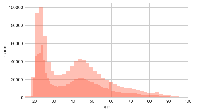
Age - as seen on graph below, it makes more sense taking people ages 18 to 30 and their mean for empty values, then people aged 31-100 and their mean for empty values;
-
New customer index - he looks at how many months customers for whom the variable is empty have, finds that they have 6 months and replaces them all by 1
-
Seniority - if lower than 0 then it is set to 0, for new customers found previously - min seniority
-
Date joined - median date is given for those for whom it’s zero
-
Status (primary/not in beginning of month) - 1 is more common so 1 for missing values
-
Client activity - replaced by median
-
City - not replaced but labeled as “UNKNOWN”
-
Renta (household income) - a lot of missing values; empty ones replaced by median by province (as incomes vary considerably across provinces in the sample)
-
Address type - dropped
-
Province code - dropped
-
Product values (dependent variables) - he looks at what was most common in previous months and replaces empty values by it
An interesting graph on age - we see that there it peaks at 24-25 (young customers) and then again at 45.
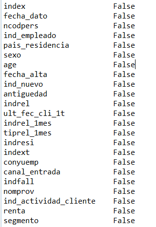
Now all the variables don’t have missing values:
print(df.isnull().any())

The model
Important - this kernel (cleaning data) does not convert text variables to numeric values, which will be a problem when/if XGBoost is used (as it works only with int, float or bool values). To solve this, numeric values are mapped onto non-numeric variables using a dictionary.
The only amendments that I’ve made are adding ‘UNKNOWN’ together with ‘NA’ and ‘’ values as it’s used in the first kernel a lot, and also removing age, seniority and renta /income of a household (as in the solution they are modified in a different way than in first kernel).
Also here the file is read with DictReader, line by line, in a way I haven’t used before. The principle is:
Read row by row → for each column take its value, match with dictionary and substitute
This is where the famous XGBoost, one of the most used and powerful algorithms in machine learning, comes in. The first model/predictions took about 20 min to make, but the score is not that high:

For the second submission I added back renta, seniority and age (although directly, not through specifying functions for each one as it’s been done in kernel 2):
x_vars = []

   for col in cat_cols:

      x_vars.append( getIndex(row, col) ) #GetIndex is a function  matching values with dictionary

      x_vars.append(int(row['age']))   #add age as it's already a number with no missing values

      x_vars.append(int(row['antiguedad']))  #add antiguedad /seniority

      x_vars.append(float(row['renta']) )  #add renta
Building model/predicting once again:
print(train_X.shape, train_y.shape)

(1071232, 39) (1071232,)

print(datetime.datetime.now()-start_time)

0:01:00.623444

print(test_X.shape)

print(datetime.datetime.now()-start_time)

(929615, 39)

0:01:32.127147

Building model..

Predicting..

0:47:28.671259

Getting the top products..

0:47:42.199612
Submit the prediction.
The prediction quality has improved, but ever so slightly.

Here, on the contrary, is the result of the forked script “When less is more” as it is result:
Almost a whole percent more (which implies that either the cleaning script, though worked well, didn’t add to the overall score, or the limitation of only June which I did outside of Python (in SQL in fact) did not work well).
