Product Client Fit

Disclaimer: The purpose of this post is to demonstrate the logic and the methodology, model choice, etc. The data has been partially generated/scrambled by the author. Demonstrated results cannot be perceived or interpreted as real data of any financial organization.

How, where, when and why clients choose financial products? This is a question managers, analysts and “conseillers d’affaires” ask themselves all the time, as this is what the revenue will ultimately depend on. Equally important is whether the client will leave, at which moment and why (as then incentives to make him stay can be found).

“Products”, as in Santander case, will be the predicted variables, and these can be anything from specific card types, to insurances, to accounts, to services for business. Here are examples of all products by a typical French bank.

It’s good to know that there are three major client categories for banks in France - particuliers, professionnels and entreprises. There are also others depending on bank policy and specification.

The data

Our train dataset is for year N while our test dataset is for the next year (N+1).
That means that when train is 2011, test is 2012, when train is 1998, test would be 1999, and so forth.

Also, as will be seen by the data, the period for train is longer than for test. For example, train - 8 months, test - 2 next months, and so forth. This is a disadvantage as train and test do not have the same length and also we are not anticipating cyclical changes (predicting June with June, like in Santander).

We take 7 products and 11 to 13 characteristics/factors that could possibly explain them.
Our goal, as in Santander challenge, is to predict whether these products will be bought or not, with maximum probability.
An important difference from Santander - in that challenge prediction was on existing customers, and here everyone in “test” dataset is new. That is to say, if the test dataset is for February and March 1999, they came into the bank in February and March 1999. In the train dataset, however, clients who are in it were with the bank before and did not come in the train period. What we are doing is basically trying to predict the behavior of new clients based on behavior of older ones.

One line is one client (not a situation where one client has several lines, thus more than one set of features). The total size of the train sample is about 30000 lines/clients, the total size of the test sample - about 8000 lines/clients. Products are anonymized, and so are features.

The data - 2

First, we can look at how the features are distributed:

for i in range(0,12):

 fig = plt.figure(figsize=(10,10))

ax = fig.add_subplot(111)

plt.yscale('log')

dataset_test[cols[i]].hist(bins=100)

dataset_train[cols[i]].hist(bins=100, ax=ax, label='train', color='blue')

#test and train are shown on the same graph

dataset_test[cols[i]].hist(bins=100, ax=ax, label='test', color='red')

legend = ax.legend()

plt.title(cols[i])

plt.yscale('log') #log scale of the axis

plt.xscale('log')

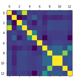
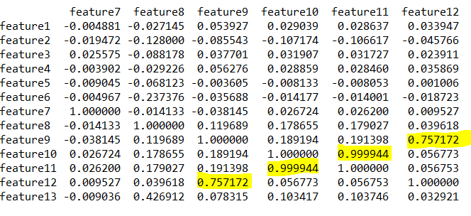
From that already we can see that most of the variables are categories - features one to 5 are. Also there’s a very strong correlation between features 10 and 11 both in test (red) and in train datasets. Also it’s visually clear that dataset for train is bigger in volumes as dataset test. Visualisation of the correlation matrix (higher correlations are highlighted):

plt.matshow(dataset_train[cols].corr()) #the correlation matrix of features

print(dataset_train[cols].corr()) #correlation values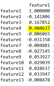

Indeed, there is a strong correlation between features 10 and 11 (they’re numerical values and nearly identical in fact), also between feature 1 and feature 4 (they are category values and so it could be that this is one category in the other or two related categories).
Also there is a strong correlation between feature 12 which is a category feature and feature 9 which is numerical.
There is something up with feature 3, too - test and train dataset are drastically different and that is why whether it’s sensible to use in in training the model.
Interesting.

For this task I’ve decided to use three models, all giving 0 or 1 as output.
The first one is Random Forest, the second one is Logistic Regression (logit) and the third one is Naive Bayes.
Cycle is probably a better solution, but they’re used consecutively on each product. Below is example for product one.

random_forest1 = RandomForestClassifier()

random_forest1.fit(X_train, Y_train_product_1.values.ravel())

Y_pred_randomforest_1 = random_forest1.predict(X_test)

print("product 1 - "+str(metrics.accuracy_score(Y_real_product_1, Y_pred_randomforest_1)) )#model score product 1

logreg = LogisticRegression()

logreg.fit(X_train, Y_train_product_1.values.ravel())

Y_pred_logreg_1 = logreg.predict(X_test)

print("product 1 - "+str(metrics.accuracy_score(Y_real_product_1, Y_pred_logreg_1)) )#model score product 1

gnb = GaussianNB()

gnb.fit(X_train, Y_train_product_1.values.ravel())

Y_pred_GNB_1=gnb.predict(X_test)

print("product 1 - "+str(metrics.accuracy_score(Y_real_product_1, Y_pred_GNB_1)) )

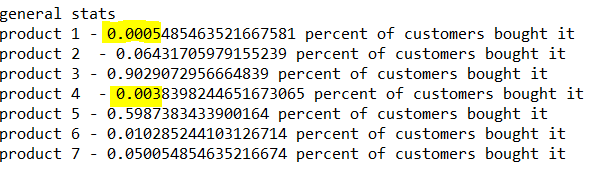
Let’s also look at the signal itself (= how many users actually bought each product in the test dataset).

print ("product 1 - "+str(sum(dataset_test["PRODUCT ONE"])/len(Y_real_product_1))+ " percent of customers bought it")

Apparently, products 1 and 4 have too small a signal to be considered. If a small percentage of clients bought the product, say, 1 in 100, if the prediction is that no clients bought the product (all 0s) is already 99% accurate…. Which is not what we want. The equivalent example is when everyone on the Titanic is dead, it’s already 60% accuracy.
On products 3 and 5 it’s the other way around - almost everyone buys them so it’s difficult to understand which predictors are important - force of the model is not that high. But we continue with them still.
Also we can remove Naive Bayes as its results are worse than two previous models.

Features importance

On product 6 the situation is most interesting - Logistic Regression gives significantly better results than Random Forest model - 0,95 against 0,88. Worth investigating further. Maybe look at the factors it takes into account?

colors=np.array(['purple', 'blue', 'r', 'pink', 'brown', 'y', 'g', 'lime', 'b', 'indigo', 'orange', 'grey','black'])

columns=np.array(['feature1', 'feature2', 'feature3', 'feature4', 'feature5', 'feature6', 'feature7', 'feature8',

 'feature9',  'feature10', 'feature11', 'feature12', 'feature13'])

features=np.array(cols)

importances6 = random_forest6.feature_importances_

indices6 = np.argsort(importances6)

plt.title('product 6 - random forest')

plt.barh(range(len(indices6)), importances6[indices6], color=colors[indices6])

plt.yticks(range(len(indices6)), features[indices6])

plt.show()

indices6_logreg = np.argsort(logreg6.coef_)

importances6_logreg=indices6_logreg[0]

#print(len(indices6_logreg), indices6_logreg[0]) #first element because it was array n an array

plt.title('product 6 - logistic regression')

plt.barh(range(13), importances6[importances6_logreg], color=colors[importances6_logreg])

plt.yticks(range(13), features[importances6_logreg])

plt.show()

Here it’s clear that the factors importance for these models is not drastically different - the weights are very close for each feature (the first graph is sorted, while the second one is not, this is why the order is different).

Let’s see for the random forest model - how important are different features for predicting each product (bearing in mind that features 10 and 11 are practically identical, and feature 3 for test dataset is very unlike train dataset).

fig, axes = plt.subplots(2,3,figsize=(16, 18))

plt.subplots_adjust(hspace=0.4, wspace=1)

#features=np.array(cols)

importances1 = random_forest1.feature_importances_

indices = np.array(np.argsort(importances1))



#one of the six graphs - product one

axes[0, 0].set_title('PRODUCT ONE')

axes[0, 0].barh(range(len(indices)), importances1[indices], color=colors[indices])

plt.sca(axes[0,0])

plt.yticks(range(len(indices)), features[indices])

Products 1-4 have a similar importance of features, while products 5 and 7 (the sixth was represented above) have a different thing going on - for product five the most important feature by far is feature3, and for product seven it’s the same but with feature4. It’s logical to assume that these products are meant for a specific client category (persioneers, young people, teenagers, travelers etc.)
It’s also notable that the most important features for majority of the products are numeric (financial) ones, thus how the client is using the offered services is in most cases more important than in what category she is.

Features engineering

As there are many categorical variables here, it’s maybe wirth generating additional variables which would be 0 or 1 for each variable, thus if, for example, feature1 has categories 23, 25, 26, then there would be new columns feature1_23, feature1_25, feature1_26 which would be 1 or 0 depending on value in feature1.

for i in feature4_unique:

 cn='feature4_' + str(i)

 cols.append(cn)

 dataset_train[cn]=np.where(dataset_train['feature4']==i,1,0)

dataset_test[cn]=np.where(dataset_test['feature4']==i,1,0)

Results (products 1 and 4 excluded as signal too feeble):

Product 2 more or less the same, products 3, 5 and 6 very slightly improved, product 7 slightly worse. Not the result we were hoping for.

The split

The last idea is to separate clients into groups using the variables provided. We could try doing it with each variable in turn and running the models on groups until they give a different enough result.
Here we will separate them by variable feature1. It could be the volume of operations each month; it could be the type - an individual or a company; it could be whether this is their main bank or not; it could be the age, as older customers do not behave and have the same tariffs as younger ones.

Here the category1 are those who have codes 68,66,67 in feature1, and category2 are those who have 64, 65, 77,91,70 or 0.

dataset_train_category1=dataset_train[(dataset_train['feature1']==68) | (dataset_train['feature1']==67) |(dataset_train['feature1']==66)]

dataset_train_category2=dataset_train[(dataset_train['feature1']==0) | (dataset_train['feature1']==64) |(dataset_train['feature1']==65)|(dataset_train['feature1']==70)|(dataset_train['feature1']==77)|(dataset_train['feature1']==91)]

dataset_test_category1=dataset_test[(dataset_test['feature1']==68) | (dataset_test['feature1']==67) | (dataset_test['feature1']==66)]

dataset_test_category2=dataset_test[(dataset_test['feature1']==0) | (dataset_test['feature1']==64) |(dataset_test['feature1']==65) | (dataset_test['feature1']==70) | (dataset_test['feature1']==77) | (dataset_test['feature1']==91)]

X_train_category1=dataset_train_category1[cols_initial]

Y_train_category1_product_2=dataset_train_category1[product_2]



n3=200

random_forest2_category1 = RandomForestClassifier(n_estimators=n3)

random_forest2_category1.fit(X_train_category1, Y_train_category1_product_2.values.ravel())

Y_pred_randomforest_2 = random_forest2_category1.predict(X_test_category1)

print("product 2 - " + str(metrics.accuracy_score(Y_real_category1_product_2, Y_pred_randomforest_2)) )

Results:

What a difference! On every single product the model works better for category 2, for some (product 3 and product five, the more “crowded” ones) significantly better.
Let’s take a look at the signal by category:

For products 2, 6 and 7 there is practically nobody buying them in category 2.
Ideas

This is by no means the end of exploration, products 3 and 5 in particular can be investigated further, but a few other ideas I’ve had (which I’ll probably describe in this blog once it’s done):

Investigate on how frequently different products are bought with each other

Limit the period of train set the same way as in Santander problem
Look at the dynamics of product buys (also similar to Santander)
Use a different algorithm (XGBoost) or a combination of a few

All the code for this task can be found on my Github.</font>

Written on April 15, 2018