Monkey Business: Predicting Volatility In The Financial Markets (from 36.7% To 25.9% Error)
Curiosity killed the cat. Also, it made me register for the challenge of predicting the volatility of selected stocks, organized this year on Challenge Data by CFM. The presentation of the challenge is available here.
This post is my first steps in analysing this purely financial dataset in the data science setting.

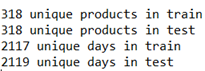
Financial datasets are very particular both in terms of models used and in particularities of the data. As Claudia Perlich, Senior Data Scientist at Two Sigma, pointed out in this video, the first thing that is extremely important is time, as these are time series data; and the second thing to think about is noise, that is to say signals within the data are not very clear. The test and train datasets are similar in size. In total, there are 318 unique products and 2117-2119 unique days (about 5,8 years of data if 365 days in a year). What is important at the first glance: This is to see whether there are many missing values and if yes, how many and in which particular columns. Here’s the number of missing values modelled (the graph “repeats itself because on the left are volatilities and on the right are returns, and where first are missing, second are too): For my first submission, I did the simplest thing - not yet modelising anything, I computed the mean of all the volatilities in each line. Submitting it as predicted volatility, here’s what I’ve got: The best top-dashboard score is 20.96%. Let’s add the model then. The simplest one is linear regression, OLS (ordinary least squares) method. Doing the prediction, replacing empty values (about 1/6 of the dataset which is, frankly, a lot) with mean ones from the previous submission, and here’s the result: Much better already. Some code can be found here.</font>
The data itself is:
- ID of each line,
- the date,
- the product id,
- volatilities for each 5-minute interval from 9-30 in the morning to 13-55 in the afternoon,
- returns for each 5--minute interval from 9-30 in the morning to 13-55 in the afternoon.
The target variable is volatility in two last hours of the day.
Here’s how the predictors look (54 periods in total for both volatilities and returns):</p>
cols = ["ID","date","product_id","volatility 09:30:00","volatility 09:35:00","volatility 09:40:00",

….

“volatility 13:40:00","volatility 13:45:00","volatility 13:50:00","volatility 13:55:00",

"return 09:30:00","return 09:35:00","return 09:40:00","return 09:45:00",

….

"return 13:40:00","return 13:45:00","return 13:50:00","return 13:55:00"]
Missing values
Here it’s clearly visible that the maximum missing values in 9-30 and 9-35 chunks (opening of the stock exchange), and also in 12-40, 12-50 and 12-55 (middle of the day). In all the other chunks, the number of missing values is relatively stable.
This is either just a particularity of the dataset, or probably these were taken out intentionally.
The max % of missing values is about 4,7%-5% which is generally good as it’s not a lot.First submission
#taking all the volatilities for each line and calculating their mean

col = input_test.loc[: , "volatility 09:30:00":"volatility 13:55:00"]
input_test['volatility_mean'] = col.mean(axis=1)
#creating a dataframe for output of a required length
output_test=pd.concat([input_test['ID'],input_test['volatility_mean']], axis=1)
Then again, I don’t have a model yet. J There’s definitely room for score improvement.
OLS method (simple linear regression)
The first problem with it is that it does not allow empty values (they have to be replaced or removed, as in the example with the ‘missing’ parameter).
The second problem with it is, obviously, correlation variables (as better to check whether columns are strongly correlated or not).#simple OLS model with a non-binary output
model = sm.OLS(output_train['TARGET'],input_train[cols], missing='drop')
results=model.fit()
output_train['TARGET1'] = results.predict(input_train[cols]) #predicting on TRAIN