The results of the competition are now official and the winners - determined, but the game Is still on, and, moreover, some solutions have been published (therefore more possibilities to improve the first, very basic, solution from previous post).  

There are many things to do with the original script, and ideas to implement, essentially:
- trying different models (other than OLS method - in published solutions I’ve seen XGBoost, Huber regression, Weighted Linear regression, LTSM, RNN, etc.)
- feature engineering (which breaks in three categories - “by ID”, “by product”, “by date” )
- separating volatilities data from returns data and treating them separately
-  ensembling / stacking

Different models that I’ve tried included linear weighted regression (as in this (https://github.com/FrancoisPierre/CFM/blob/master/Starting_kit.ipynb ) baseline solution), XGBoost and Huber regression (both mentioned in http://datachallenge.cfm.fr/t/proposed-solution/105 this solution).
For the last two - I am surely not tuning them in a correct way, as their results for me are far from those mentioned in the article, and even quite far from weighted linear regression, for that matter.

For now the returns are completely dropped out of prediction (as with them for this model the prediction is way worse then just with volatilities).
Finally, the most important part is generation of new features based on “ID” dimension. The “basic” are:

• Mean volatility,

• Max volatility,

• Min volatility,

• Standard deviation (or “volatility of volatility”, as it’s called in pdf above),

• Median volatility.

The non-basic ones are:

• Accumulated volatility per ID - calculated as SUM(V*P), where V, P are vectors of volatility and price for morning day ticks

• Price up max per ID - maximal volatility jump at a sequential price increase

• Price down max per ID - maximal volatility jump at a sequential price decrease

• Price up total per ID - total volatility in price up ticks

• Price down total per ID - total volatility in price down ticks

• Price up average per ID - average volatility in price up ticks

• Price down average per ID - average volatility in price down ticks

• Maximal asymmetry per ID - (Price up max - Price down max)/(Price up max + Price down max)

• Total asymmetry per ID - (Price up total - Price down total) / (Price up total + Price down total)

• Total average asymmetry per ID - (Price up average - Price down average) / (Price up average + Price down average

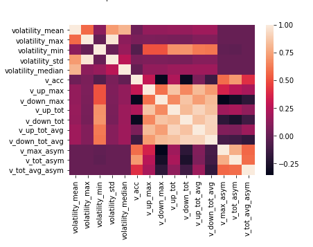
Worth looking at correlations of these variables with each other:

It’s clearly visible that the block of “up and down” calculated variables has higher intercorrelations, and so do total and max asymmetry, consequently.
Thus, the new prediction is made with all the volatilities and the newly generated variables.
Weighted linear regression:

Here the interpolation is not used, the missing values are just filled by 0 (as when the interpolation is used first for this model, the prediction quality goes down to 23.729 instead of 23.43 which it gives when missing values are just replaced by zeros).
The highest the OLS method (previously used) gives is 24.22.  

Even though returns are not used for the predictions, it’s possible to generate some new variables with returns as well:

• Returns up per ID - number of ticks where the return goes up (of “+1”s)

• Returns down per ID - number of ticks where the return goes down (of “-1”s)

• Asymmetry of returns - (Returns up - Returns down) / (Returns up + Returns down)

Of course, I’ve been trying other models and specifications as well and noticing some things:

• For XGBoost, the highest result I’ve obtained is 26.96

• XGBoost seems to work a lot better with interpolation than without it (gives 27.87 with missing values just replaced by 0)  (?)

• The question of depth of the tree/overfitting and tuning in XGBoost remains open

• For Huber regression, I’ve got MAPE as high as 70.47 (?) for the most basic specification

• XGBoost using both returns and volatilities works better than Weighted regression using returns and volatilities (its results suffer, while for XGB they improve)

Some further thoughts In terms of modelisation:

• Features importance graph is needed

• Certain features can be added still

Skewness and kurtosis (per ID) - idea of first place solutions here (https://github.com/cyrilledelabre/cfm-challenge/blob/master/CFM-Challenge-Example-Model.ipynb)
Number of NaN variables (per ID)
The “return_i = volatility_i * return sign_i” idea introduced in solution place 5 http://datachallenge.cfm.fr/t/proposed-solution/105 - it has to be noted that accumulated volatility variable reflects the principle, but it’s the total one, not “9:30”, “9:35”, “9:40” variables
Average of first three volatilities (beginning of day, solution 5)
Average of last six volatilities (end of afternoon, solution 5)
Difference / spread between afternoon and opening - this is already partially reflected in additional variables; but not quite in a way solution 5 introduces it
Computing returns of market (averaging all stocks) and volatilities of market (per each day?) - solution 5
Computing correlations between returns of every single stock with returns on the whole market , volatilities of every single stock with volatilities of market (per day?)  - solution 5
“Product” dimension (distinct days per product, max and min volatility per product) - from place 1 solution
“Day” dimension (distinct products per day, …) - from place 1 solution

+ Anything to be done with the outliers?

Finally, the submitted result is 22.96 on test, thus the mode has actually performed better on test then it did on train (23.4). A pleasant, albeit unexpected, surprise.